VideoCube Benchmark: Dataset
We provide a high-quality, large-scale benchmark VideoCube for this novel GIT task. It consists of 500 long-term videos with 7.4M frames that covers different object classes, scenario types, motion modes, and challenge attributes, with an average length of 14920 frames.

Multiple collection dimension - 6D Principle
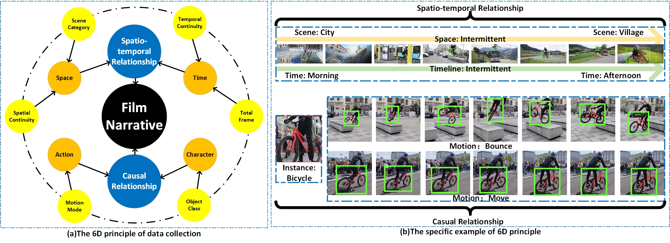
The collection of VideoCube is based on six dimensions to describe the spatio-temporal relationship and causal relationship of film narrative, which provides an extensive dataset for the novel GIT task. We guarantee that each video contains at least 4008 frames, and the average frame length in VideoCube is around 14920. Besides, the selected videos contain transitions and target disappearance-reappearance process to cancel the motion continuity assumption.

We split the film's narrative into the spatio-temporal and causal relationship and further decompose them into six dimensions (scene category, spatial continuity, temporal continuity, total frame, motion mode, object class) to provide a more comprehensive description of a video.

The figures above illustrate the data distribution of VideoCube and LaSOT.We believe that the 6D principle provides a scientific guide for the data collection, which increases the richness of video content and helps users quickly restore the narration from the six elements, improving the practicality of VideoCube.
Specific annotation principle and exhaustive checkout flow
A professional labeling team manually marked each video with a 10Hz annotation frequency, and all videos have passed three rounds of review by trained verifiers. Based on rigorous experiments, we selected the most effective algorithm to combine manual annotations and accomplish further intensive labels with 30Hz frequency.
Comprehensive attribute selection
Multiple shots and frequent scene-switching make the video content changes dramatically and become more challenging for algorithms. Thus, we accommodate twelve attributes annotations for each frame to implement a more elaborate reference for the performance analysis.
VideoCube Benchmark: Evaluation System
The evaluation system aims to judge the capabilities of the model (such as accuracy and robustness) through a reasonable evaluation method.
Traditional protocol: One-pass evaluation (OPE)
The OTB benchmark defines one-pass evaluation (OPE) as using the ground-truth in the first frame to initialize the model and locating the target in subsequent frames continuously.
Novel protocol: One-pass evaluation with restart mechanism (R-OPE)
The restart mechanism is essential in evaluating the GIT task based on the following reasons:
- Videos in VideoCube have a longer average frame and include multiple challenging characteristics like shot-switching and scene-transferring. Thus, models are prone to fail in locating instances and cannot be reinitialized.
- The count of restarts can be quantified as an indicator to measure the robustness of the algorithm.

The first row illustrates the traditional OPE mechanism. In the first frame, the tracker is initialized, and the algorithm result (blue) and ground-truth (red) coincide. The IoU value of the algorithm result (blue) and ground-truth (red) is less than a threshold (usually 0.5) in the 130th frame, indicates a failure. However, the OPE mechanism does not detect the algorithm failure, the continued failure causing subsequent frames to be wasted.
The second row is the R-OPE mechanism with failure detection and tracker restart. The green frame indicates an appropriate restart point. After the tracking failure is detected at frame 130, the algorithm will be re-initialized at the nearest restart point (frame 132), and subsequent sequences will continue to participate in the evaluation. When the tracking failure occurs in frame 281, the algorithm will be restarted at frame 282.
VideoCube Benchmark - Evaluation Metrics
The performance measurement focuses on quantitatively mapping the model capabilities through the scientific calculation to accomplish more in-depth analysis and sort the results via numerical values.
Precision plot
Tradition precision (PRE) measures the center distance between the predicted result $p^t$ and the ground-truth $b^t$ in pixels. Calculating the proportion of frames whose distance is less than the specified threshold and drawing the statistical results based on different thresholds into a curve generates the precision plot. Typically, trackers are ranked on 20 pixels.

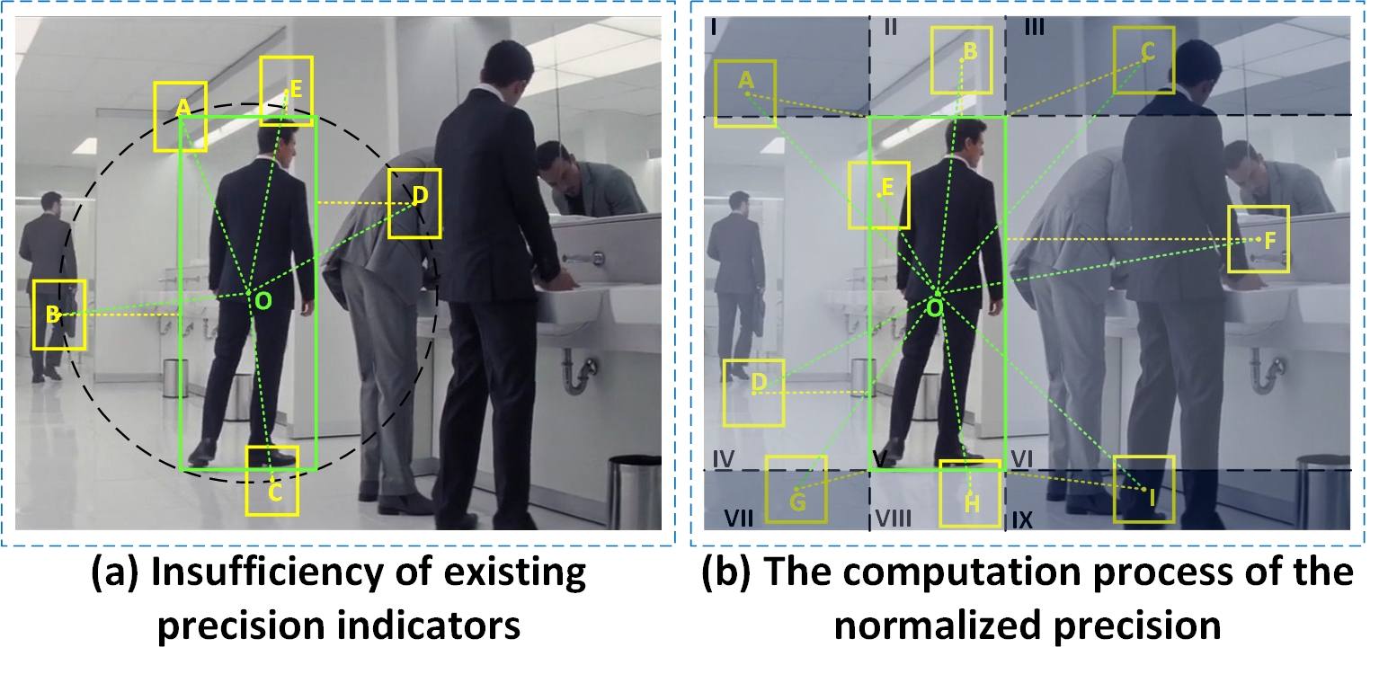
Figure (a) presents a counterexample. The green rectangle represents the ground-truth, where point $O$ denotes the center point. Assume that five yellow rectangular boxes show the prediction results of the five algorithms. To eliminate the influence of other factors, here assumes the prediction results have only position differences. $OA$, $OB$, $OC$, and $OD$ are the same, while $OE$ is slightly larger. The precision scores of tracker $A$, $B$, $C$, $D$ based on two existing metrics (directly using the center point distance or only using the current ground-truth size for normalization) are the same, while tracker $E$ is worse. Nevertheless, from the Figure (a), we can directly judge that $A$ and $E$ perform better than $B$. The calculation results are contrary to the common sense because the target aspect ratio affects accuracy but is ignored by existing metrics. For non-square bounding boxes, only the center point distance cannot quantify the tracking accuracy accurately.
In order to deal with the above this problem, we propose a new precision metric N-PRE. Explicitly, we select the center distance as the original precision if the tracker center point falls into the ground-truth rectangle. Algorithms with predicted center outside the ground-truth rectangle will also calculate the shortest distance between its center and the ground-truth edge. As shown in the Figure (b), the original precision value of tracker $E$ is $OE$, while other trackers are calculated by two parts (center distance represented by the green dashed line, and the penalty item represented by the yellow dashed line). Subsequently, we quantify the original precision value to the $[0,1]$ interval; 0 represents the tracker center point is $O$, while 1 represents the score of the farthest point in the current frame (upper right point). In the Figure (a), the performance of tracker $A$ evaluated via N-RPE is the best while tracker $B$ is the worst. It is consistent to the reality.
Success plot
To get the success rate (SR), we first calculate the Intersection over Union (IoU) of the predicted result $p^t$ and the ground-truth $b^t$. Frames with an overlap rate greater than a specified threshold are defined as successful tracking, and the SR measures the percentage of successfully tracked frames under different overlap thresholds. The statistical results based on different thresholds create the success plot. Besides, we implement two more success plots based on Generalized IoU (GIoU) and Distance IoU (DIoU), aiming to provide a comprehensive scientific evaluation.